Principal component analysis: pictures, code and proofs
The code used to generate the plots for this post can be found here.
I.
Principal component analysis is a form of feature engineering that reduces the number of dimensions needed to represent your data. If a neural network has fewer inputs then there are less weights to train, which makes it easier and faster to train the model.
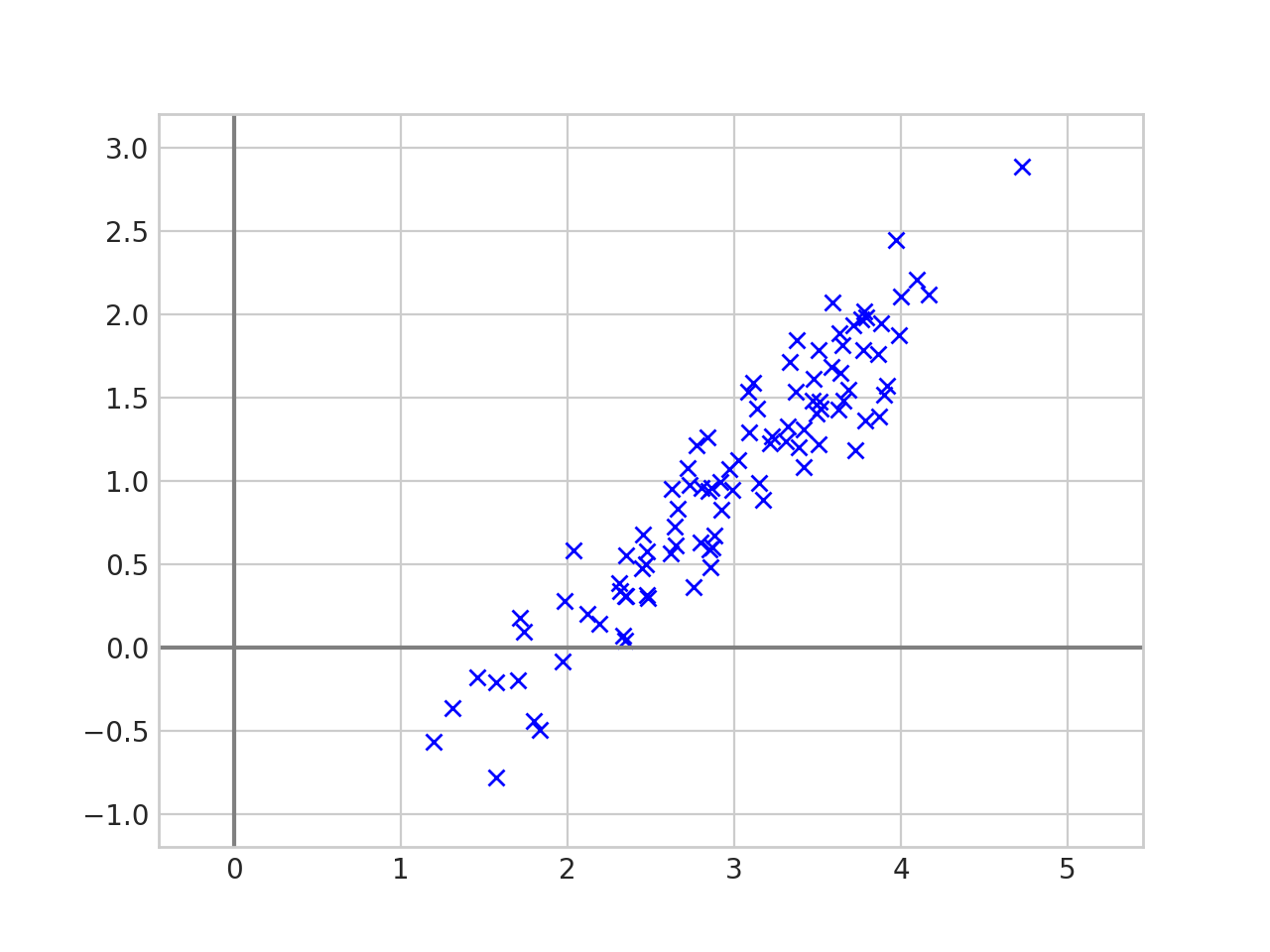
The data above is two dimensional, but it is “almost” one dimensional in the sense that every point is close to a line.
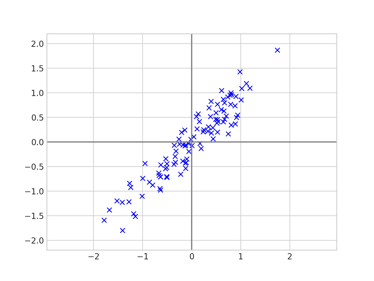
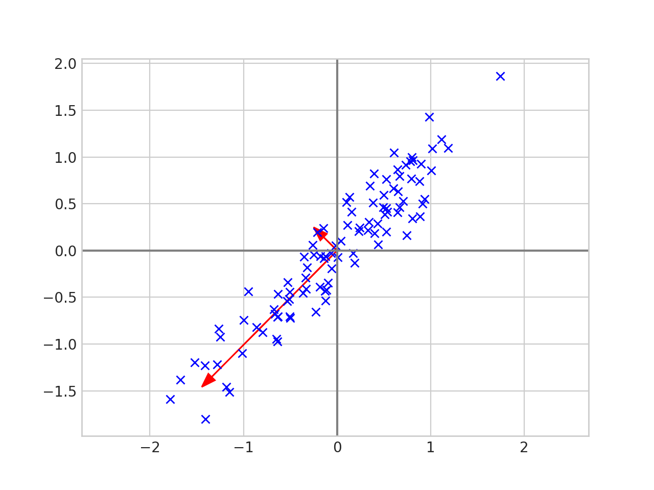
The first step in principal component analysis is to center the data. Given the list of 2d points, \(x_1, x_2, \dots , x_n \in \mathbb{R}^2\) we first center the data by calculating the mean \(\overline{x} = \frac{1}{n}\sum_{i=1}^n x_i\) and replacing each \(x_i\) with \(x_i - \overline{x}\). Now the data looks like this.
We then put the data in a matrix \(X = \begin{pmatrix} | & | & & | \\ x_1 & x_2 &\cdots & x_n \\ | & | & & |\end{pmatrix}.\) And calculate the eigenvectors and eigenvalues of the covariance matrix \(\frac{1}{n-1}XX^\top\).
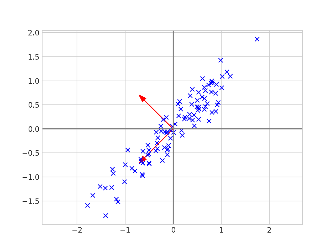
The eigenvectors tell us the direction of the data. The first eigenvector in the picture above has the same slope as the data and the second eigenvector is perpendicular to the first. Now let’s scale each of the eigenvectors by its corresponding eigenvalue 1.
And draw an ellipse around the eigenvectors.
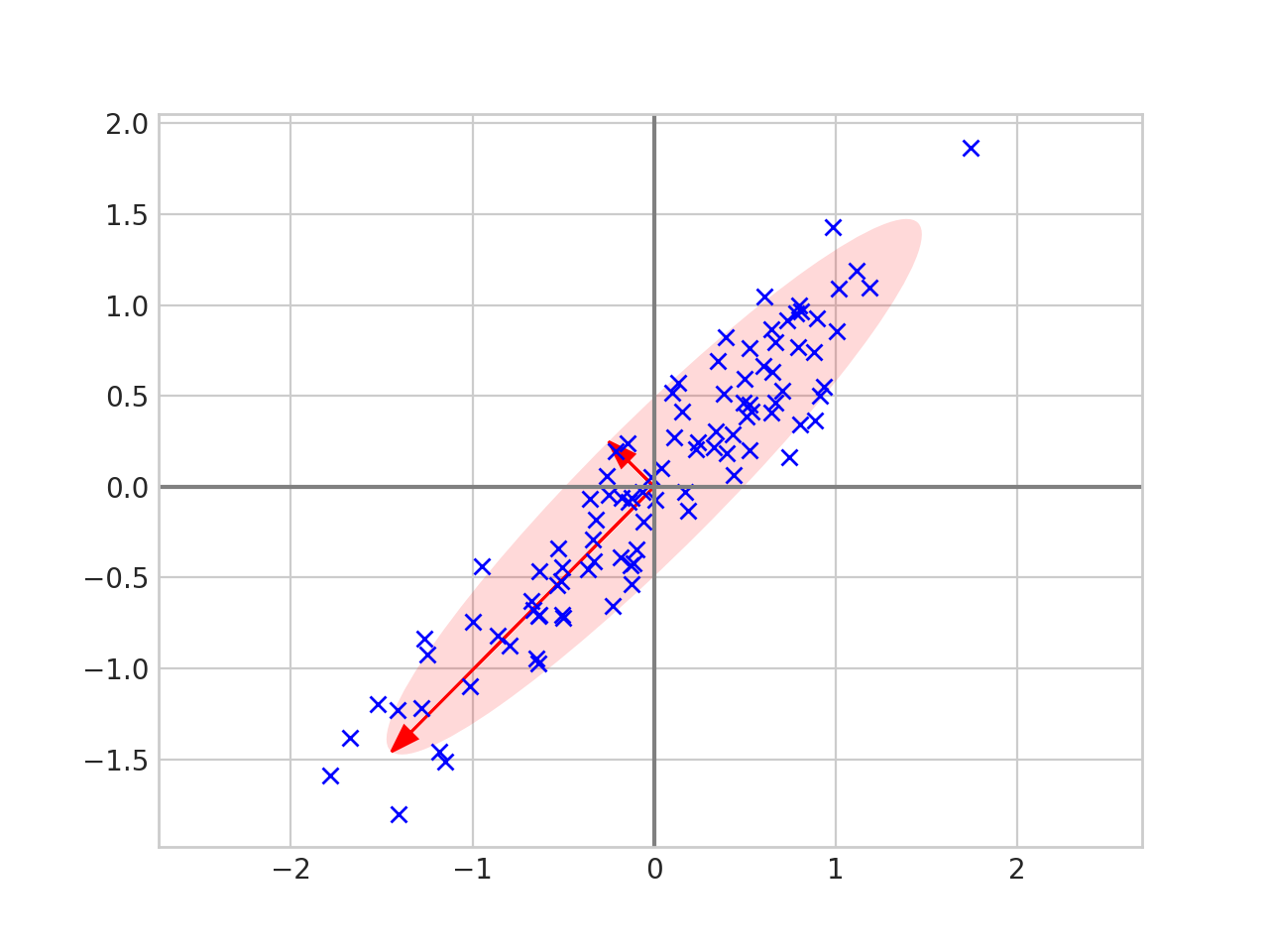
The eigenvalues tell us how spread out the data is in the direction of that particular eigenvector. Thus we can reduce the dimension of the data by projecting onto the line given by the largest eigenvalue.
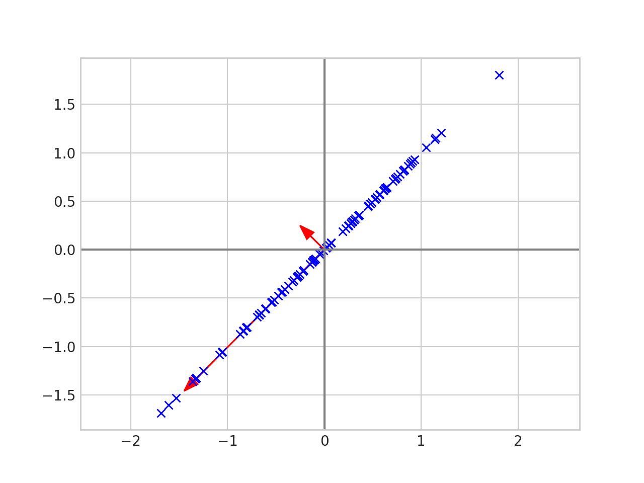
The data is now one dimensional since it fits on a single line. Each point has not moved too far from its original spot, so these new points still represent the data well.
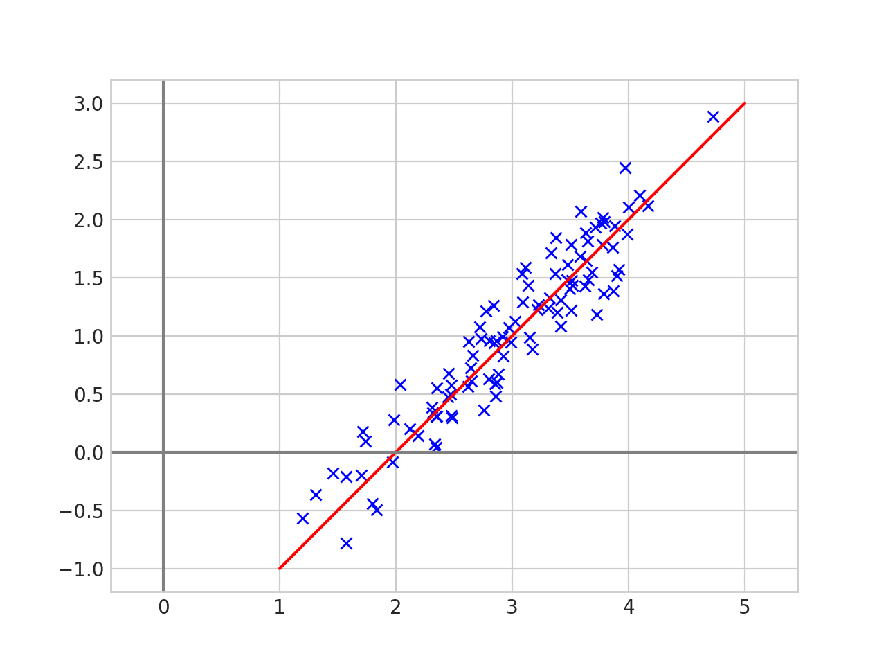
In two dimensions this is the same as projecting onto the line of best fit, but this technique generalizes. If your data is \(n\)-dimensional then PCA lets you find the best \(m\)-dimensional subspace to project the data down onto; you just project your data onto the subspace spanned by the \(m\) eigenvectors with the largest eigenvalues. If \(m < < n\) this can compress your data a lot, and PCA guarantees that this \(m\) dimensional subspace is optimal, in the sense that it minimizes the mean squared error between the original data points and the projected data points.
II.
The data in the plots above was generated using a random number generator. Let’s try PCA on a real dataset.
We will use the MNIST dataset, which is a collection of grayscale, 28x28 images of hand written digits. To simplify the analysis we will discard images of 2,3,4,5,6,7,8,9 and only look at images of 0 and 1. Below are some examples of the images from MNIST.
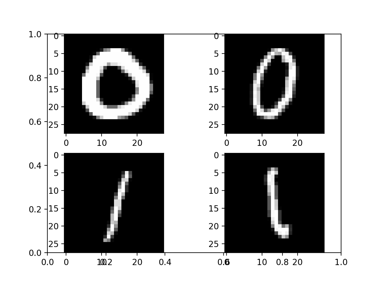
To process the images we will:
- Flatten each image into a \(784 = 28\times 28\) dimensional vector.
- Use PCA to project each 784-dimensional vector to a 2-dimensional vector.
- Plot the 2 dimensional vectors, with images of ‘0’ in red and images of ‘1’ in blue.
The result looks like this.
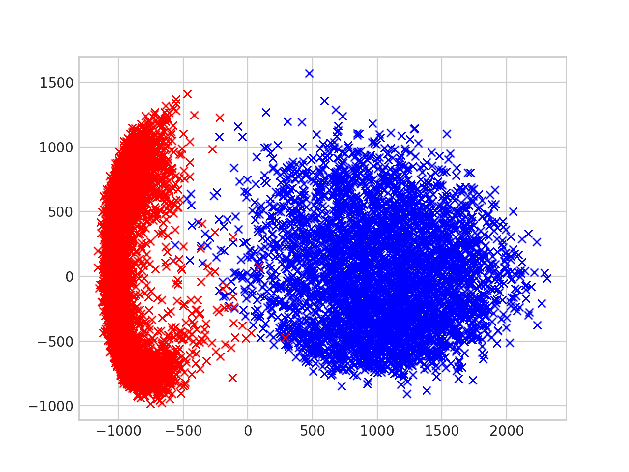
You can see that the zeros are clustered to the left, and the ones are clustered to the right. We could create a reasonable classifier by drawing a vertical line at \(x = - 250\), and all we did was linearly project the raw pixels down to a two dimensional subspace!
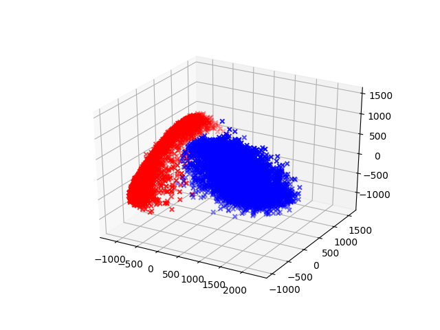
We can project onto any number of dimensions. Here is the three dimensional projection.
III.
It’s not obvious why the eigenvalues and eigenvectors of the covariance matrix have all these useful properties. There are proofs at the end of the post, but they’re not particularly enlightening. Thankfully there’s a more intuitive way of thinking about it.
Continuing with the MNIST example, let \(p_1\) be the vector where the \(i\)-th entry is the first pixel in the \(i\)-th image. Simlarly let \(p_2, p_3, \dots , p_{784}\) be the vectors consisting of the 2nd, 3rd … , 784th pixels across all images. Then
\[XX^\top = \begin{pmatrix} \langle p_1, p_1 \rangle & \langle p_1, p_2 \rangle & \cdots & \langle p_1, p_{784} \rangle \\ \langle p_2, p_1 \rangle & \langle p_2, p_2 \rangle & \cdots& \langle p_2, p_{784} \rangle \\ \vdots & \vdots & \ddots & \vdots \\ \langle p_{784}, p_1 \rangle & \langle p_{784}, p_2 \rangle & \cdots & \langle p_{784}, p_{784} \rangle \\ \end{pmatrix}.\]This matrix can be diagonalized \(XX^\top = UDU^{-1}\) where \(U\) is a change of basis matrix and \(D = \operatorname{diag}(\lambda_1, \cdots , \lambda_n)\) is diagonal. We can view the change of basis as creating new features \(p_1’, p_2’, \dots , p_{748}’\) from the original pixels. And the diagonal matrix is the covariance matrix for these new features.
Since \(\langle p_i’, p_j’ \rangle = 0\) for \(i \neq j\) the features are independent, and the variance of \(p_i’\) is \(\langle p_i’, p_i’ \rangle = \lambda_i\).
So given a vector of pixels \(x\), we can convert \(x\) into a vector of new features \(x’\) by applying a change of basis. Then the eigenvalues \(\lambda_i\) are the variances of the new features, it seems reasonable that the features with the largest variance are the most important, while the features with the smallest variance can be discarded.
IV.
Now that we have some intuition, the preceding discussion can be formalized into a theorem.
Theorem: Let \(x_1, \dots , x_n \in \mathbb{R}^d\) be a sequence of data points. Let
\[X = \begin{pmatrix} | & | & & | \\ x_1 & x_2 &\cdots & x_n \\ | & | & & |\end{pmatrix}\]be the \(d \times n\) matrix where each column is a data point. Let \(W = XX^\top\) (the \(\frac{1}{n-1}\) factor from before does not affect the eigenvectors or the relative order of the eigenvalues). Then \(W\) is positive semidefinite and hence has eigenvectors \(u_1, \dots , u_d\) which form an orthonormal basis for \(\mathbb{R}^d\). Let \(\lambda_1, \dots , \lambda_d\) be the corresponding eigenvalues and without loss of generality assume \(\lambda_1 \geq \lambda_2 \cdots \geq \lambda_d\). The projection error for \(x_i\) onto a subspace \(V \subset \mathbb{R}^d\) is defined as \(\|x_i - P_Vx_i\|_2^2\) where \(P_V:\mathbb{R}^d \to \mathbb{R}^d\) is the projection-onto-\(V\) operator. Then for any positive integer \(m < d\) the subspace \(U_m := \operatorname{span}\{u_1, \dots , u_m\}\) minimizes the sum of the projection errors. In symbols,
\[\sum_{i=1}^n \|x_i - P_{U_m}x_i\|_2^2 = \min_{\substack{V \subset \mathbb{R}^d \\ \operatorname{dim}V = m}} \sum_{i=1}^n \|x_i - P_Vx_i\|_2^2.\]Proof:
Fix \(m < d\) and let \(V \subset \mathbb{R}^d\) be an \(m\)-dimensional subspace. Define the \(d \times n\) error matrix \[ E = \begin{pmatrix} | & | & & |\\ x_1 - P_Vx_1 & x_2 - P_Vx_2 & \cdots & x_n - P_Vx_n\\ | & | & & | \\ \end{pmatrix} = X - P_VX. \] We want to minimize \[ \sum_{i=1}^n \|x_i - P_Vx_i\|_2^2 = \|E\|_F^2 \] where \(\|\cdot \|_F\) is the Frobenius norm. We now rewrite the error using matrix algebra \[ \begin{align}\newcommand{\tr}{\mathrm{tr}} \|E \|_F^2 &= \| X- P_VX\|_F^2 \\ &=\tr\left(( X- P_VX)( X- P_VX)^\top\right) & (\|A \|_F^2 = \tr(A^\top A)) \\ &=\tr\left(( X- P_VX)( X^\top - X^\top P_V^\top)\right) \\ &=\tr\left(XX^\top - XX^\top P_V^\top - P_VXX^\top + P_VXX^\top P_V^\top \right) \\ &=\tr\left(W- W P_V^\top - P_VW + P_VW P_V^\top \right) & (W = XX^\top)\\ &=\tr\left(W- W P_V - P_VW + P_VW P_V \right) & (P_V = P_V^\top )\\ &=\tr(W)- \tr(W P_V) - \tr(P_VW) + \tr(P_VW P_V ) \\ &=\tr(W)- \tr(P_VW ) - \tr(P_VW) + \tr(P_VW) & (\tr(AB) = \tr(BA) \text{ and } P_V^2 = P_V)\\ &=\tr(W)- \tr(P_VW). \end{align} \]
The quantity \(\mathrm{tr}(W)\) is a constant, so minimizing \(\|E \|_F^2\) is the same as maximizing \(\tr(P_VW)\). Let \(\{v_1, \dots , v_m\} \subset \mathbb{R}^d\) be an orthonormal basis for \(V\). Then \[ P_V = \sum_{i = 1}^m v_iv_i^\top \] so \[ \begin{align}\newcommand{\tr}{\mathrm{tr}} \tr(P_VW) &= \tr\left(\sum_{i = 1}^m v_iv_i^\top W \right) \\ &= \sum_{i=1}^m \tr\left(v_iv_i^\top W\right) \\ &= \sum_{i=1}^m \tr(v_i^\top W v_i) & (\tr(AB) = \tr(BA)). \end{align} \]
Let \[ U = \begin{pmatrix} | & | & & | \\ u_1 & u_2 &\cdots & u_d \\ | & | & & |\end{pmatrix} \] where the \(u_i \in \mathbb{R}^d\) are the eigenvectors of \(W\) as stated in the theorem. The matrix \(U\) diagonalizes \(W\) so \(W = UDU^{-1} = UDU^\top\) where \[D = \begin{pmatrix} \lambda_1 & 0 & \dots & 0 \\ 0 & \lambda_2 & \dots & 0 \\ \vdots & \vdots & \ddots & \vdots \\ 0 & 0 & \dots & \lambda_n \end{pmatrix}. \] Now \[ \begin{align}\newcommand{\tr}{\mathrm{tr}} \tr(P_VW) &= \sum_{i=1}^m \tr(v_i^\top W v_i) \\ &= \sum_{i=1}^m \tr(v_i^\top UDU^\top v_i) \\ &= \sum_{i=1}^m \tr((U^\top v_i)^\top D (U^\top v_i) \end{align} \]
If \(v_i = u_i\) for all \(1 \leq i \leq m\) then \[U^\top v_i = U^\top u_i = (0, \dots, 0, 1, 0, \dots, 0)^\top\] is the \(i\)-th standard basis vector. Thus \[ \begin{align}\newcommand{\tr}{\mathrm{tr}} \tr(P_VW) &= \sum_{i=1}^m \tr((U^\top v_i)^\top D (U^\top v_i) \\ &= \sum_{i=1}^m \lambda_i \end{align} \]
Therefore it suffices to show that \(\mathrm{tr}(P_VW) \leq \sum_{i=1}^m \lambda_i\) for all dimension \(m\) subspaces \(V\).
We will show this is true in the case \(m = 2\), i.e. \(\mathrm{tr}(P_VW) \leq \lambda_1 + \lambda_2\) when \(V\) is 2 dimensional. The case \(m > 2\) uses the same argument but it is more notationally heavy. Let \(\alpha = U^\top v_1 \in \mathbb{R}^d\) and \(\beta =U^\top v_2 \in \mathbb{R}^d\). Note that since \(U\) is unitary \(\|\alpha\|_2^2 = \|\beta\|_2^2 = 1\) and \(\langle \alpha, \beta \rangle = 0\).
The first step is to show that \(\alpha_i^2 + \beta_i^2 \leq 1\) for all \(i\). Let \(e_i = (0, \dots , 0, 1, 0, \dots , 0)\) be the \(i\)-th standard basis vector. Since \(\alpha\) and \(\beta\) are orthogonal and have length 1, the projection of \(e_i\) onto \(\operatorname{span}\{\alpha, \beta \}\) is given by \[\hat{e}_i = \langle e_i, \alpha \rangle \alpha + \langle e_i, \beta \rangle \beta = \alpha_i \alpha + \beta_i \beta .\] Then \[ \alpha_i^2 + \beta_i^2 = \|\hat{e_i}\|_2^2 \leq \|e_i\|_2^2 = 1 \] since a projected vector always has length less than or equal to the original vector.
The second step is to observe that \(\sum_{i=1}^d (\alpha_i^2 + \beta_i^2) = \|\alpha \|_2^2 + \|\beta \|_2^2 = 2\).
Finally, we want to maximize \[ \mathrm{tr}(P_VW) = \sum_{i=1}^d \lambda_i(\alpha_i^2 + \beta_i^2) \] and we know that \[\alpha_i^2 + \beta_i^2 \leq 1 \text{ and } \sum_{i=1}^d(\alpha_i^2 + \beta_i^2) = 2 .\]
The eigenvalues of a positive semidefinite matrix are nonnegative so the sum \(\sum_{i=1}^d \lambda_i(\alpha_i^2 + \beta_i^2)\) is maximized when when the first and second coefficient are as large as possible, i.e. when \(\alpha_1^2 + \beta_1^2 = \alpha_2^2 + \beta_2^2 = 1\). But then the second condition implies that \(\alpha_i^2 + \beta_i^2 = 0\) for \(i > 2\). Thus \[ \mathrm{tr}(P_VW) = \sum_{i=1}^d \lambda_i(\alpha_i^2 + \beta_i^2) \leq \lambda_1 + \lambda_2. \] \(\square\)
We also need to prove that the size of the eigenvalue is proportional to the variance in the direction of the corresponding eigenvector.
Theorem: As in the previous theorem let \(X = \begin{pmatrix}x_1 & x_2 & \cdots & x_n \end{pmatrix}\) be the data matrix, \(W = XX^\top\) the covariance matrix, \(u_1, \dots , u_d\) the eigenvectors of \(W\) and \(\lambda_1, \dots , \lambda_d\) the eigenvalues. Let \(P_{u_i}: \mathbb{R}^d \to \mathbb{R}^d\) be the projection operator onto the subspace \(\mathrm{span}\{u_i\}\). Then \[ \sum_{j=1}^m\|P_{u_i}x_j\|_2^2 = \lambda_i \]
Proof:
The working is similar to the previous proof so I'll omit some steps. \[ \begin{align} \sum_{j=1}^m\|P_{u_i}x_j\|_2^2 &= \|u_iu_i^\top X\|_F^2 \\ &= \mathrm{tr}((u_iu_i^\top X)(u_iu_i^\top X)^\top) \\ &= \mathrm{tr}(u_i^\top W u_i) \\ &= \mathrm{tr}((U^\top u_i)^\top D (U^\top u_i) \\ &= \lambda_i . \end{align} \]
1 I actually scaled by two times the square root of the eigenvalue. The eigenvalue tells you the variance and I wanted the standard deviation. I multiplied by two so that ellipse would capture most of the data. ↩